BKD trees, used in Elasticsearch
I had worked on Elasticsearch back in 2015, when it was more known for its text searching capabilities using inverted indexes. As I looked to pick it up again last year for another project, I saw that Elasticsearch had added core support for other data types from text like numbers, IP addresses, geospatial data types, etc.
As I looked to understand the main differences which could allow optimized search over such data types, I stumbled upon BKD trees. Surprisingly, there is not much written about BKD trees apart from a white paper and some blogs. The blog post will look to cover elements leading up to the development of BKD trees and its advantages starting from KD trees.
We will start with the BST (Binary Search Tree) which will be the base for our post. A BST is a binary tree which has lesser elements to its left and greater elements to its right for all nodes. The article will not contain more information regarding the insertion, deletion and searching of elements further since there are numerous sources out there.
BST or other similar implementations of BST like AVL trees, leverage the capability of dividing the search space by 2 at each node during the traversal, thus resulting in a O(logN) search in the best case scenario. It is possible to balance BSTs by rotating the tree with the pivot.
A major flaw or lack of ability with the BST is the ability to deal with multiple dimensions or spaces. For example, if we have a store of latitudes and longitudes, and we are asked to search for a specific set of latitude and longitude. It is easy for us to use BST to search for either the latitude or longitude but not both the elements together since BST is capable of handling only one dimension in its store.
What do we do if we have multiple dimensions or multiple metrics across which we need to run our search queries?
KD or K-Dimensional trees#
This is where KD or K-Dimensional trees come into the picture. KD trees are similar to BST in the terms that it allows segregation of data to the left or right depending on the value. The main difference is the consideration of multiple planes or dimensions or spaces while constructing it. In a KD tree or K-NN problems, each traversal is able to divide a particular plane into 2 equal sub planes. As the traversals go deeper, the combination of division of planes is used to reach the point in space that was being searched for.
A very good example of splitting of planes in a 1 dimensional structure is the binary search method on an array. For every jump, half of the array is taken out of consideration.
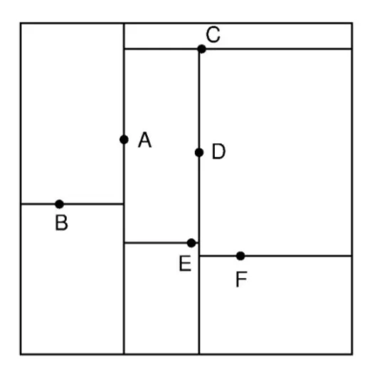
For a 2D structure, the structure can be split in the following way:

For the point A, the X axis is split into 2. For the point B and C, the Y axis is split into 2 and so on.
How do we represent the 2D split in a tree?
In order to do this, we define something called as the discriminator. The discriminator is mainly used to figure out which plane is to be considered for the split during the jump. The formula to figure out the discriminator is
discriminator = level % N, where level is the level of the tree and N is the number of dimensions
Each dimension is assigned a key. The key is used against the discriminator value of each node.

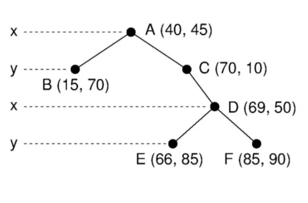
We will try to use the above knowledge to try to explain the tree.
At node A, discriminator = 0 % 2 = 0
At node B, discriminator = 1% 2 = 1
At node C, discriminator = 1% 2 = 1
At node D, discriminator = 2 % 2 = 0
At node E, discriminator = 3 % 2 = 1
At node F, discriminator = 3 % 2 = 1
Since there are only 2 dimensions here, the discriminator value can be only 0 or 1 since the level starts from 0. We will call the first dimension as X and the second dimension as Y. The X can very well be the latitude and Y the longitude.
Applying BST strategy here, we select the next node based on the comparison of values of the dimension.
Let us try to search the element with value S(66, 85)
At point A, discriminator is 0, hence we compare the X dimension of S and A. S(X) is 66 and A(X) is 40. Since 66 > 40, we navigate to the right which is the C node.
At point C, discriminator is 1, hence we compare the Y dimension of S and A. S(Y) is 85 and C(Y) is 10. Since 85 > 10, we navigate to the right which is the D node.
At point D, discriminator is 0, hence we compare the X dimension of S and A. S(X) is 66 and D(X) is 69. Since 66 < 69, we navigate to the left which is the E node.
We finally reach the node that we were searching for.
The same algorithm can be used to a 3D or a 4D structure as well. The only change is the calculation of the discriminator and the number of discriminator values will be 3 or 4 respectively depending on the dimensions. If it’s a 3D structure, the space will repeat itself every 3 jumps.
As we can see above, the read operations tend to be optimized well keeping N-dimensions in mind.
Any insertion or deletion on the tree can be a little more tricky than in a BST. In a BST, the rotation works since we are rotating along only one dimension. Rotation in a KD tree will not work easily since rotation along only one dimension will disrupt the other dimensions as well. Hence, write operations on a KD tree can become expensive.
In the above example, the space division selection is done in a round robin fashion. However, that is the simplest approach that can be taken to ensure proper cutting of all spaces. If we want to give more priority to specific dimensions, it can very easily be controlled by modifying the discriminator formula to reflect the same.
The BKD tree is a collection of multiple KD trees as children. This makes sense as the write operation propagations can be controlled to a single KD tree as the data increases. Since BKD trees were mainly built for disk operations, it borrows a leaf (pun intended) from B+ trees and stores the actual points only at the leaf nodes. The internal nodes are mainly used as pointers to reach the appropriate blocks. The tree is a combination of complete binary trees and B+ trees. Since it is a complete binary tree, array techniques using formulas like 2n+1 and 2n+2 can be used to fetch the appropriate child nodes which will be further optimized for disk IO. I have a hunch that the number of KD trees and the nodes in them can be directly correlated with the shard sizes used in Elasticsearch.
Searching on a N-dimensional space#
In this section, we try to use the above learnt knowledge of developing the required atomic query types using which other complex queries can be built.
- Filter based on X dimensions where 1 <= X <= N
- Top hits based on X dimensions as the unique scope on a function of Y dimensions where 1 <= X <= N and and 1 <= Y <= N
- Range distribution or buckets formation with X dimensions as the unique scope on a function of Y dimensions falling within defined ranges where 1 <= X <= N and and 1 <= Y <= N
- Temporal listing of X dimensions with sampling functions performed on Y dimensions where 1 <= X <= N and and 1 <= Y <= N
- Datatable listing of X dimensions where 1 <= X <= N
I think being able to restrict the queries to be a collection of the above query types should be enough to answer further complex queries.
References